PNG

PNG (Portable Network Graphics) is a well-known image format for storing image data using lossless compression.

First up, let's cover the most exciting part of the PNG format: Filters.

Filters

In order to achieve smaller compression sizes, PNG supports a variety of ways that the current pixel can be represented, and these representations are calculated based on the filtering algorithm being used.

The 5 types of PNG filters are:

• None
• Sub
• Up
• Average
• Paeth

Even more interesting is that each filter is applied per-scanline, meaning that you can have all 5 filters being used at once in a single PNG image, as is usually the case. By mixing filters, you can achieve varying pixel representations for each scanline, which can significantly reduce the compressed size of the file.

This is because PNG uses the DEFLATE compression algorithm – but instead of going into the LZ77 algorithm and Huffman coding, just know that repeated values are better for compression. By using certain filters on certain scanlines, you can make it so that more of these repeated patterns appear, thus improving the compression rate and decreasing the overall size of the file.

But why is this information important for our purposes? Let's jump right in and explore filters a bit more.

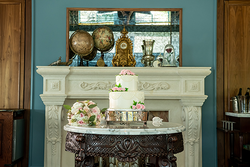
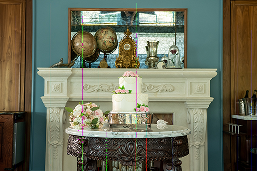
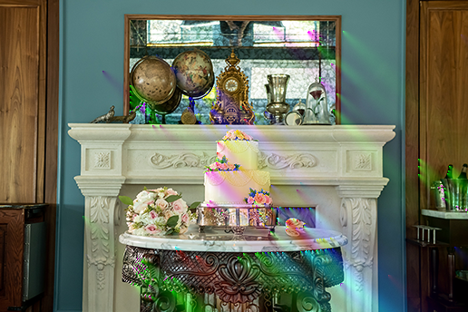
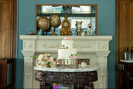
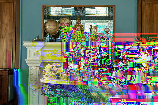
I'll be using this image to show the filter effects.

Filter: None

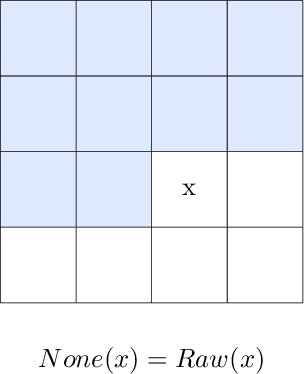
The None algorithm stores RGB values as their raw values – in other words, no filtering is done at all.

Altering data when using the None filter is literally just bopping raw R/G/B values and is pretty boring. You might change a purple pixel to a green one or something.

Like, just look at this.

Looks pretty similar to the original image, right?

Here are a few of the differences.

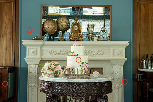
There are actually 20 bytes that were replaced in the image. Can you find them all?

Additionally, while the None algorithm may be mostly boring, it does introduce some pretty cool possibilities when you remove bytes intead of simply replacing them.

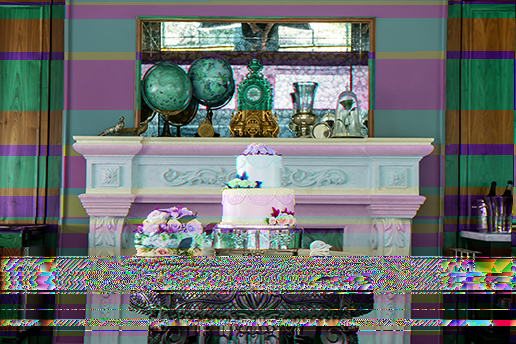
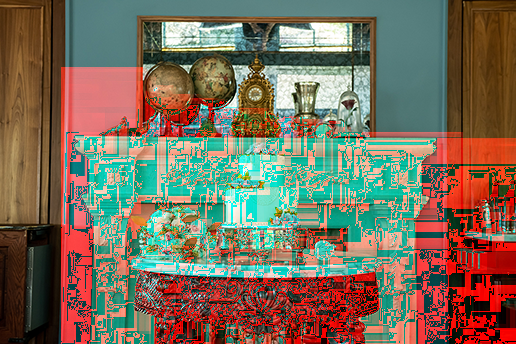
Filter: Sub

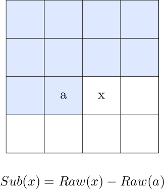
The Sub algorithm stores the difference between the current pixel's R/G/B value and the left pixel's R/G/B value.

Altering data using the Sub filter means that every pixel to the right of the altered pixel will also have its value altered in some way.

This one is pretty fun to experiment with, but the output is usually somewhat predictable.

Things really start to get interesting when the output of the Sub algorithm is modified. For example, when applying a binary AND mask to the result, you start to get these kinds of outputs.

Filter: Up

The Up algorithm stores the difference between the current pixel's R/G/B value and the upper pixel's R/G/B value.

Altering data using the Up filter means that ever pixel below the altered pixel will also have its value altered in some way.

This is pretty similar to the Sub filter, except just going vertical instead of horizontal.

As with Sub, things start to get really neat once you start playing with the algorithm's output value. This is probably one of the ones I enjoy the most, since applying a binary AND mask to these (especially 0xFE) makes the color look like the color's bleeding downwards.

Filter: Average

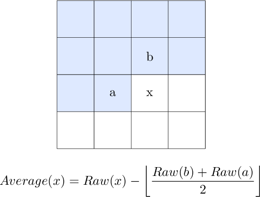
The Average algorithm calculates the average of the left pixel's R/G/B value and the upper pixel's R/G/B value, then subtracts that average from the current pixel's R/G/B value.

Okay, now this one's pretty neat. Altering data using the Average filter affects the pixels below it and to the right of it, creating what appears to be a fading diagonal "spray" of color, with the most intense colors occurring near the source of the altered pixel.

Interestingly, even though only 20 bytes were modified, the "sprays" from the altered R/G/B values can sometimes create entirely new pixels that initiate a "spray" of their own.

Since this algorithm is somewhat more complex than the previous algorithms, there are more opportunities to introduce modifications to the algorithm.

First, let's explore what happens if you apply a modified Average filter (Up -> mask -> Average) to the 1st pixel of each row, then apply the normal Average filter to every other pixel.

This effect is relatively tame since only the 1st pixel of each row is modified. However, it shows that modifying the algorithm does have some controlled effect on the resultant output.

Now let's look at what happens when you apply a mask to the normal output of the Average filter.

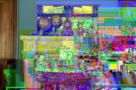
Filter: Paeth

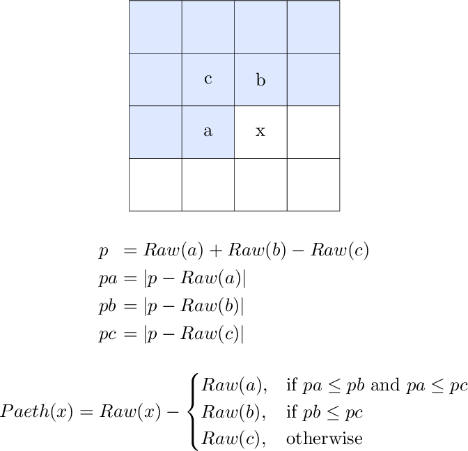
The Paeth algorithm is pretty complex compared to the other algorithms.

First, it makes an initial estimate by adding the left pixel's R/G/B value and the upper pixel's R/G/B value together, then subtracting the upper-left pixel's R/G/B value.

The absolute value of this estimate relative to each of its components is then calculated, effectively marking its "distance" to each component.

At this point, the Paeth algorithm chooses whichever is closest to it: The left pixel, the upper pixel, or the upper-left pixel.

Finally, the R/G/B value of the closest pixel is subtracted from the current pixel's R/G/B value.

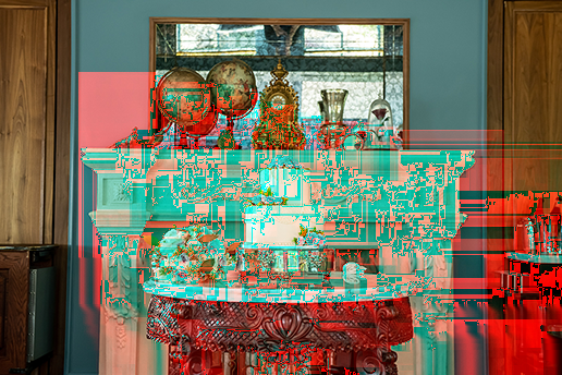
Altering data using the Paeth algorithm has perhaps the most chaotic effects right out of the gate, as modifying even a single pixel can have extreme block-like effects on all pixels to the right of it and below it.

Similar to the Average filter, this algorithm is also significantly more complex than None, Sub, and Up, meaning there's many more opportunities to introduce modifications to the filtering algorithm.

Like Average, let's explore what happens when applying a modified Paeth filter (Up -> mask -> Paeth) to the 1st pixel of each row, then apply the normal Paeth filter to every other pixel.

Pretty trippy. But if you look closely, you can see that the structure of the image is still there, even through all the wild colors.

However, applying a mask to the normal output of the Paeth filter provides a much different result.

Filter: Optimized

While this isn't actually a filtering algorithm in itself, it still deserves to be highlighted as a potential for some fun experimentation.

When you save a PNG from an image editing program, chances are that it'll attempt to optimize the PNG to at least some extent in order to reduce the filesize.

Remember that filters are applied per-scanline. Because no single filtering algorithm is best for every use case, a combination of filters is typically used in order to achieve better compression rates.

Additionally, tools such as OptiPNG can further attempt to find improved compression opportunities to further reduce the filesize.

For example, let's take a look at what changing 1 single R/G/B value looks like when applied to a PNG exported by Photoshop.

You can see that most of the scanlines are utilizing Paeth, but there's an Average filter being applied starting somewhere around scanline 236.

Let's see what happens when we run that same PNG through OptiPNG and change another R/G/B value around that same area.

Oddly enough, it looks like OptiPNG decided on using Paeth full through. And that's not OptiPNG just being lazy.

In fact, OptiPNG managed to shear off 912 bytes by using Paeth exclusively, which results in a 0.29% decrease in file size.

Altering data when the file is using software-determined optimized filters can really show how the edits to one scanline can Æffect all of the others below it.

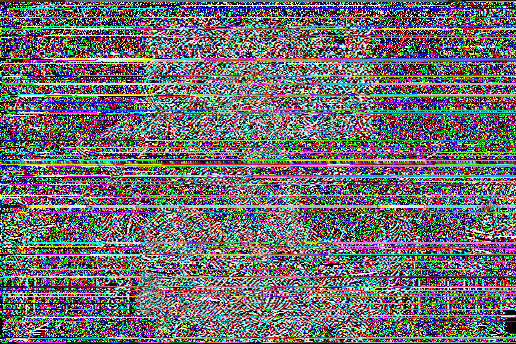
Filter: Random

To wrap up filters, here's what happens if you randomly change only the first byte of every scanline while leaving every other byte intact, which will result in a random filter being specified for every scanline.

Compression

Don't worry, I'm not going into detail about DEFLATE, LZ77, or Huffman coding. Instead, the focus here is on the relation of compression to the PNG file format as a whole.

In order to achieve smaller file sizes, the data for each IDAT chunk (which holds image data) is compressed using the DEFLATE algorithm.

This is very important to note because modifying data post-compression is not the same as modifying data prior to compression.

When modifying data before compression, the modified data is written to the scanline and then compressed. This means that when the file is decompressed, the modified data is read just fine, as expected.

However, when modifying data after compression, the data that gets read will almost always be different than how it was initially written due to the way DEFLATE decompresses (AKA inflates) the compressed data.

Even changing just 1 byte in a compressed IDAT chunk can have catastrophic effects on the rest of the image.

First, here's a relatively tame outcome that was achieved when modifying 1 byte of the compressed data relatively late in the file.

Not too bad. I dig the little rainbow effect going on there at the bottom.

What about changing 1 byte around the middle or so of the compressed data?

This kind of looks similar to how we replaced 20 bytes (before compression) with optimized filters, except we only changed 1 byte in the compressed data.

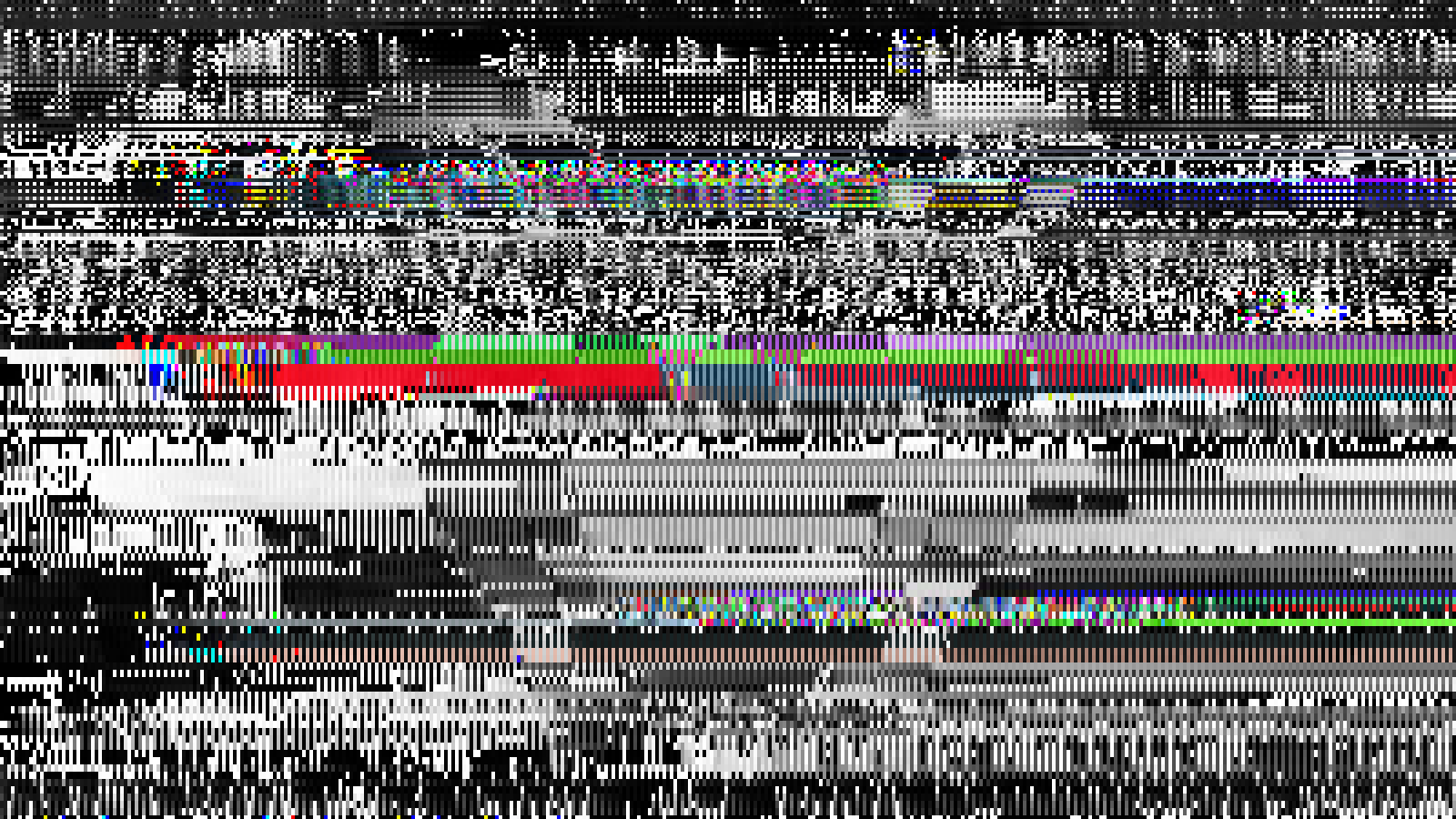
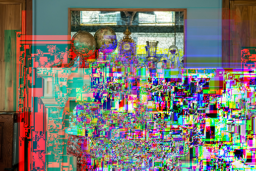
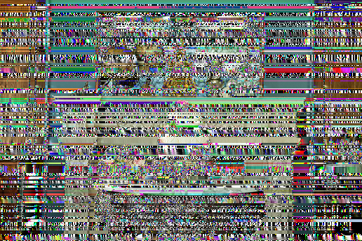
Now let's see what happens when a byte is replaced very early in the compressed data.

As you can see, a good amount of care must be taken when modifying PNG data post-compression, as doing so can really mess up a lot of the image.

Interlacing

If you've ever tried to load an image using a bad internet connection, you've seen that it can sometimes take a while to load.

Have you noticed that some images load from the top-down, while others are loaded very blurry and gradually un-blur?

We're going to be focusing on that 2nd technique, which is achieved through interlacing.

By interlacing data, you can show more of the image faster while giving the browser time to load the complete image.

Let's take a look at this clock in the image.

When saving data in PNG format, you have the option of interlacing the data using the Adam7 algorithm, which is a 7-step process that fills in dots of data at a time (although these show up as blocks in the browser).

The video below shows the general theory of how interlacing works.

Now that we know how Adam7 interlacing works at a conceptual level, understanding how images are gradually displayed at the browser-level is fairly simple.

Instead of just adding colored dots to the image, browsers instead take the dot's color and fill in an entire block of color. By doing this, the browser makes sure there are no blank spots between the "dots" as the image loads.